MODULE_06 // SIGNAL_INTELLIGENCE

SIGNAL_INTELLIGENCE // RF_ANALYSIS_GUIDE

This technical handbook supports identification and analysis of unusual radio frequencies (RF anomalies) in biologically relevant ranges. We cover the full chain here: from selecting the right hardware and software through to correctly interpreting signal traces and initial indications of possible relationships.

[ DETECTION_LOG: SIGNAL-ANALYSIS-GUIDE ]

This section is a practical working guide for precise RF measurements. Here you learn which devices you actually need, how to minimize intrusive self-generated signals from your environment, and how to reliably separate transmit energy (the carrier wave) from the actual information signals (modulation).

1. HARDWARE // THE SDR TOOLCHAIN

Professional measurements require a dedicated software-defined radio (SDR) receiver, a matched antenna, and high-quality shielded cables. Only this hardware combination makes weak signals visible and lets you distinguish real RF activity precisely from technical self-noise.

HACKRF ONE
This is the central tool for this workflow. HackRF One covers an enormous frequency range and delivers detailed raw data (IQ data), so even fine modulation patterns become visible in analysis software.
Advantage: High detail depth and exact repeatability of measurements.
Important note: Internal gain should be set moderately to avoid overload and artificial ghost signals (aliasing).
ANTENNEN
The antenna acts as a filter to the outside world. While a broadband antenna is helpful for the first overview, detailed analysis should switch to a band-matched antenna optimized for the target range.
Problem: If antenna geometry does not match the frequency, weak signals disappear into the noise even though they are physically present.
SMA / HOST HYGIENE
Connection quality is often underestimated. Poor SMA cables behave like antennas for interference from laptops or USB ports.
Recommendation: Use short, double-shielded cables and high-quality adapters.
Extra protection: A USB isolator can help suppress electrical hum and unwanted side lines right at the computer.

2. SOFTWARE // PYTHON & DESKTOP-SDR

Programs such as SDR++, GQRX, or SDR Angel provide initial orientation: they deliver a live waterfall for visually monitoring frequencies. For deeper forensic analysis—especially to document envelope structure or temporal signal evolution—automated evaluation via Python is significantly more precise. Our script delivers reproducible data that goes beyond visual estimation alone.

PYTHON // UNIFIED RF HELPER (PSD + ENVELOPE + SPEC)

To standardize signal analysis, we use a combination of SoapySDR, NumPy, and Matplotlib. This toolchain lets you capture raw data directly from the SDR and process it mathematically.

Modes: The script can be configured flexibly via --mode:

psd: Power spectral density analysis to locate signals in the frequency spectrum.
envelope: Visualization of modulation patterns in the low-frequency range (e.g., timed pulses).
both: Runs PSD and envelope analysis together without the spectrogram—useful for faster passes or when you want less plotting overhead than --mode all.
spectrogram: Time–frequency representation for documenting temporal stability of a signal.
all: Generates all analyses at once in one overview.

Robustness: The CLI helper processes streams stably, reduces read errors through automatic retries, and uses window functions (Hann window) to minimize measurement error.

Download targeting-humans_rf_analysis.py

#!/usr/bin/env python3
# -*- coding: utf-8 -*-
"""
================================================================================
  Targeting Humans — RF capture helper (PSD + envelope + spectrogram)
================================================================================

  ZWECK / PURPOSE
  ----------------
  Dieses EINZEL-Skript ersetzt zwei frühere Varianten und führt sie zusammen:

    (A) Kurze FFT über IQ → grobe Leistungsdichte (PSD) um die Mittenfrequenz
    (B) Betrag der IQ-Samples (= instantane Amplitude / Hüllkurve) → FFT davon
        → zeigt, welche *Modulationsfrequenzen* im Niederfrequenzbereich im Signal
            stecken (z. B. kHz-Bereich), sofern sie im erfassten Zeitfenster
            stabil genug sind.

  WICHTIG / IMPORTANT
  -------------------
  • Nur empfangen, wenn ihr dazu berechtigt seid (Genehmigungen, Ortsrecht).
  • RF-Sicherheit: keine ungeeigneten Antennen an Leistungs-PEP anschließen.
  • Das Skript ist LEHR-/DEMONSTRATIONSZWECK — keine Garantie auf Messgenauigkeit.

  ABHÄNGIGKEITEN / DEPENDENCIES
  ------------------------------
    pip install numpy matplotlib SoapySDR

  Zusätzlich: passender SoapySDR-Modul-Treiber für euer Gerät, z. B.:
    • HackRF: SoapyHackRF + libhackrf
    • Andere SDRs: jeweils deren Soapy-Plugin installieren und --driver anpassen

  BEISPIEL / EXAMPLE
  ------------------
    python targeting-humans_rf_analysis.py --freq-hz 780e6 --rate 2e6 --mode all

    python targeting-humans_rf_analysis.py --freq-hz 2.44e9 --rate 10e6 --mode envelope --no-plot

================================================================================
"""

from __future__ import annotations

import argparse
import json
import sys
import traceback
from typing import Any, Optional, Tuple

# -----------------------------------------------------------------------------
# Optionale Abhängigkeiten — klare Fehlermeldungen, falls etwas fehlt
# -----------------------------------------------------------------------------
try:
    import numpy as np
except ImportError as exc:  # pragma: no cover
    print("FEHLER: numpy fehlt. Install: pip install numpy", file=sys.stderr)
    raise SystemExit(1) from exc

try:
    import matplotlib.pyplot as plt
except ImportError as exc:  # pragma: no cover
    print("FEHLER: matplotlib fehlt. Install: pip install matplotlib", file=sys.stderr)
    raise SystemExit(1) from exc

def _require_soapy() -> Any:
    """Importiert SoapySDR nur bei Hardware-Capture-Pfaden."""
    try:
        import SoapySDR  # type: ignore
    except ImportError as exc:  # pragma: no cover
        print(
            "FEHLER: SoapySDR (Python-Binding) fehlt.\n"
            "  Install (Beispiel): pip install SoapySDR\n"
            "  Außerdem müssen die nativen Soapy-Module + Gerätetreiber installiert sein.",
            file=sys.stderr,
        )
        raise SystemExit(1) from exc
    return SoapySDR


# =============================================================================
# Hilfsfunktionen / helpers
# =============================================================================


def _parse_device_args(raw: str) -> str:
    """
    Soapy akzeptiert oft JSON-Strings oder key=value-Ketten.
    Wir erwarten hier JSON wie: {"driver":"hackrf"}
    """
    raw = raw.strip()
    if not raw:
        return json.dumps({"driver": "hackrf"})
    # Wenn der Nutzer schon gültiges JSON liefert, durchreichen
    try:
        json.loads(raw)
        return raw
    except json.JSONDecodeError:
        # Fallback: als driver-String interpretieren
        return json.dumps({"driver": raw})


def open_device(soapy: Any, device_args: str) -> Any:
    """Öffnet genau ein Soapy-Gerät; bei Fehler: lesbare Meldung."""
    try:
        return soapy.Device(device_args)
    except Exception as exc:  # noqa: BLE001 — Soapy wirft diverse Typen
        print(
            "\n=== GERÄT KONNTE NICHT GEÖFFNET WERDEN ===\n"
            f"device_args = {device_args!r}\n"
            "Tipps:\n"
            "  • Ist das Gerät per USB eingesteckt?\n"
            "  • Läuft eine andere App (SDR++, GQRX), die den Dongle blockiert?\n"
            "  • Stimmt der Treiber? Test: SoapySDRUtil --find\n",
            file=sys.stderr,
        )
        traceback.print_exc()
        raise SystemExit(2) from exc


def configure_rx(
    soapy: Any,
    sdr: Any,
    sample_rate: float,
    center_hz: float,
    gain_db: Optional[float],
) -> None:
    """Grundlegende RX-Konfiguration (Kanal 0)."""
    # Sample-Rate setzen — manche Geräte quantisieren; Soapy snapped ggf. automatisch
    sdr.setSampleRate(soapy.SOAPY_SDR_RX, 0, float(sample_rate))
    sr_actual = sdr.getSampleRate(soapy.SOAPY_SDR_RX, 0)
    if abs(sr_actual - sample_rate) / max(sample_rate, 1.0) > 0.05:
        print(
            f"HINWEIS: angeforderte Sample-Rate {sample_rate:.0f} Hz, "
            f"Gerät nutzt {sr_actual:.0f} Hz.",
            file=sys.stderr,
        )

    sdr.setFrequency(soapy.SOAPY_SDR_RX, 0, float(center_hz))

    if gain_db is not None:
        # Viele Geräte: overall gain; falls nicht unterstützt, ignoriert Soapy ggf. still —
        # dann manuell im SDR-Utility prüfen.
        try:
            sdr.setGain(soapy.SOAPY_SDR_RX, 0, float(gain_db))
        except Exception:  # noqa: BLE001
            print(
                "WARNUNG: setGain schlug fehl — Gain manuell im Treiber prüfen.",
                file=sys.stderr,
            )


def _read_stream_result(ret) -> int:
    """Soapy Python-Binding: Rückgabe ist meist Objekt mit .ret, ältere APIs ggf. int."""
    if hasattr(ret, "ret"):
        return int(ret.ret)
    return int(ret)


def capture_iq_burst(
    soapy: Any,
    sdr: Any,
    num_samps: int,
    timeout_us: int,
    max_retries: int,
) -> Tuple[np.ndarray, float]:
    """
    Nimmt einen IQ-Block auf (komplex float32).

    Returns
    -------
    samples : (N,) complex64
    sample_rate : float — tatsächliche Rate nach Geräte-Snap
    """
    rx_stream = sdr.setupStream(soapy.SOAPY_SDR_RX, soapy.SOAPY_SDR_CF32)
    sdr.activateStream(rx_stream)

    buff = np.zeros(int(num_samps), dtype=np.complex64)
    sr_actual = float(sdr.getSampleRate(soapy.SOAPY_SDR_RX, 0))

    try:
        total = 0
        for attempt in range(max_retries):
            ret = sdr.readStream(
                rx_stream,
                [buff[total:]],
                len(buff) - total,
                timeoutUs=int(timeout_us),
            )
            nread = _read_stream_result(ret)
            if nread > 0:
                total += nread
            elif nread == soapy.SOAPY_SDR_TIMEOUT:
                print(
                    f"WARNUNG: Timeout bei readStream (Versuch {attempt + 1}/{max_retries}).",
                    file=sys.stderr,
                )
            elif nread == soapy.SOAPY_SDR_OVERFLOW:
                print("WARNUNG: Overflow — Sample-Rate oder Host-Last zu hoch.", file=sys.stderr)
            else:
                print(f"WARNUNG: readStream ret={nread}", file=sys.stderr)

            if total >= len(buff):
                break

        if total < len(buff):
            print(
                f"WARNUNG: nur {total} von {len(buff)} Samples erhalten — "
                "Plots können verrauscht sein.",
                file=sys.stderr,
            )
            # Rest bleibt Null — besser als Abbruch für Demozwecke
        return buff, sr_actual
    finally:
        sdr.deactivateStream(rx_stream)
        sdr.closeStream(rx_stream)


def psd_from_iq(iq: np.ndarray, sample_rate: float, window: bool) -> Tuple[np.ndarray, np.ndarray]:
    """
    Einfache PSD-Schätzung aus einem IQ-Block (nicht Welch — nur Demo).

    window=True → Hann-Fenster reduziert spektrales Leck (Leakage).
    """
    x = iq.astype(np.complex64, copy=False)
    n = len(x)
    if n < 8:
        raise ValueError("Zu wenige Samples für FFT.")

    if window:
        w = np.hanning(n).astype(np.float32)
        x = x * w
        # Coherent gain Kompensation (approx)
        scale = float(np.sum(w**2) / n)
    else:
        scale = 1.0

    spec = np.fft.fftshift(np.fft.fft(x))
    psd = (np.abs(spec) ** 2) / (n * max(scale, 1e-12))
    freqs = np.fft.fftshift(np.fft.fftfreq(n, d=1.0 / float(sample_rate)))
    return freqs, psd


def envelope_modulation_spectrum(
    iq: np.ndarray,
    sample_rate: float,
    max_mod_hz: float,
) -> Tuple[np.ndarray, np.ndarray]:
    """
    |IQ| → reellwertiges Signal → rFFT → Magnitude.

    Das zeigt Energie in *Modulationsfrequenzen* bis max_mod_hz (theoretisch bis fs/2,
    wir schneiden für Lesbarkeit oft bei einigen 10 kHz / 50 kHz ab).
    """
    env = np.abs(iq.astype(np.complex64, copy=False))
    env = env - float(np.mean(env))  # DC-Anteil im Envelope reduzieren (vereinfacht)
    n = len(env)
    spec = np.fft.rfft(env)
    freqs = np.fft.rfftfreq(n, d=1.0 / float(sample_rate))
    mag = np.abs(spec)

    mask = freqs <= float(max_mod_hz)
    return freqs[mask], mag[mask]


def spectrogram_from_iq(
    iq: np.ndarray,
    sample_rate: float,
    nfft: int,
    noverlap: int,
) -> Tuple[np.ndarray, np.ndarray, np.ndarray]:
    """
    Zeit-Frequenz-Darstellung aus I-Komponente (Basisband).

    Hinweis: Für die Website-Demo reicht ein robuster, einfacher Spectrogramm-Blick.
    """
    x = np.real(iq.astype(np.complex64, copy=False))
    if nfft < 64:
        nfft = 64
    if noverlap >= nfft:
        noverlap = nfft // 2
    # Matplotlib liefert f (Hz), t (s), Sxx.
    sxx, freqs, times, _ = plt.specgram(
        x,
        NFFT=int(nfft),
        Fs=float(sample_rate),
        noverlap=int(noverlap),
        mode="magnitude",
        scale="dB",
    )
    plt.clf()  # temporäre Figure aus specgram-Helferaufruf bereinigen
    return freqs, times, sxx


def synthetic_iq_burst(
    num_samps: int,
    sample_rate: float,
    mod_hz: float,
    noise_std: float,
) -> Tuple[np.ndarray, float]:
    """
    Simulierter IQ-Block für hardwarelosen Selbsttest.
    Enthält:
      - konstante Träger-Amplitude
      - sinusförmige Amplitudenmodulation bei mod_hz
      - komplexes weißes Rauschen
    """
    n = int(num_samps)
    t = np.arange(n, dtype=np.float32) / float(sample_rate)
    carrier = np.exp(1j * np.zeros(n, dtype=np.float32))
    envelope = 1.0 + 0.25 * np.sin(2.0 * np.pi * float(mod_hz) * t)
    iq = (envelope.astype(np.float32) * carrier).astype(np.complex64)
    if noise_std > 0:
        noise = (np.random.normal(0.0, noise_std, n) + 1j * np.random.normal(0.0, noise_std, n)).astype(
            np.complex64
        )
        iq = iq + noise
    return iq.astype(np.complex64), float(sample_rate)


def build_arg_parser() -> argparse.ArgumentParser:
    p = argparse.ArgumentParser(
        description="Unified PSD + envelope/modulation spectrum capture (SoapySDR).",
        formatter_class=argparse.ArgumentDefaultsHelpFormatter,
    )
    p.add_argument(
        "--device-args",
        type=str,
        default='{"driver":"hackrf"}',
        help='Soapy device args as JSON string, e.g. \'{"driver":"hackrf"}\'',
    )
    p.add_argument("--freq-hz", type=float, required=True, help="Center frequency in Hz (e.g. 780e6).")
    p.add_argument(
        "--rate",
        type=float,
        default=2e6,
        help="Sample rate (Hz). Lower rates are easier on USB/CPU.",
    )
    p.add_argument("--fft-size", type=int, default=4096, help="Number of IQ samples per capture.")
    p.add_argument(
        "--gain-db",
        type=float,
        default=None,
        help="Optional RX gain in dB (if supported by the device).",
    )
    p.add_argument(
        "--mode",
        choices=("psd", "envelope", "spectrogram", "both", "all"),
        default="all",
        help="Which plot(s) to generate.",
    )
    p.add_argument(
        "--max-mod-hz",
        type=float,
        default=50e3,
        help="Max modulation frequency to show in envelope spectrum (Hz).",
    )
    p.add_argument(
        "--no-hann",
        action="store_true",
        help="Disable Hann window on IQ before PSD FFT (more leakage, sharper transients).",
    )
    p.add_argument(
        "--timeout-us",
        type=int,
        default=500_000,
        help="readStream timeout per call (microseconds).",
    )
    p.add_argument(
        "--retries",
        type=int,
        default=5,
        help="How many readStream attempts to fill the buffer.",
    )
    p.add_argument(
        "--save",
        type=str,
        default=None,
        help="If set, save figure to this path (PNG) instead of showing a window.",
    )
    p.add_argument(
        "--no-plot",
        action="store_true",
        help="Do not display or save plots (capture self-test only).",
    )
    p.add_argument(
        "--selftest-sim",
        action="store_true",
        help="Use synthetic IQ data instead of SDR hardware (CI/offline self-test).",
    )
    p.add_argument(
        "--selftest-mod-hz",
        type=float,
        default=9.25e3,
        help="Modulation tone for synthetic IQ self-test (Hz).",
    )
    p.add_argument(
        "--selftest-noise-std",
        type=float,
        default=0.02,
        help="Noise std-dev for synthetic IQ self-test.",
    )
    p.add_argument(
        "--spec-nfft",
        type=int,
        default=256,
        help="Spectrogram FFT size (samples per window).",
    )
    p.add_argument(
        "--spec-overlap",
        type=int,
        default=192,
        help="Spectrogram overlap (samples).",
    )
    return p


def main() -> int:
    args = build_arg_parser().parse_args()
    device_args = _parse_device_args(args.device_args)

    if args.fft_size < 256:
        print("FEHLER: --fft-size zu klein (min 256 empfohlen).", file=sys.stderr)
        return 3

    if args.selftest_sim:
        iq, sr = synthetic_iq_burst(
            num_samps=args.fft_size,
            sample_rate=args.rate,
            mod_hz=args.selftest_mod_hz,
            noise_std=args.selftest_noise_std,
        )
    else:
        soapy = _require_soapy()
        sdr = open_device(soapy, device_args)
        try:
            configure_rx(soapy, sdr, sample_rate=args.rate, center_hz=args.freq_hz, gain_db=args.gain_db)
            iq, sr = capture_iq_burst(
                soapy,
                sdr,
                num_samps=args.fft_size,
                timeout_us=args.timeout_us,
                max_retries=args.retries,
            )
        finally:
            # Device-Destruktor; explizit del in neueren Soapy-Versionen nicht nötig
            del sdr

    if args.no_plot:
        source = "simulated IQ" if args.selftest_sim else "SDR capture"
        print(f"OK: {len(iq)} Samples @ {sr:.0f} Hz ({source}) complete.")
        return 0

    modes = []
    if args.mode in ("psd", "both", "all"):
        modes.append("psd")
    if args.mode in ("envelope", "both", "all"):
        modes.append("env")
    if args.mode in ("spectrogram", "all"):
        modes.append("spec")

    nplots = len(modes)
    fig, axes = plt.subplots(nplots, 1, figsize=(10, 3.5 * nplots), squeeze=False)
    ax_list = axes.ravel()

    plot_idx = 0
    if "psd" in modes:
        ax = ax_list[plot_idx]
        plot_idx += 1
        freqs, psd = psd_from_iq(iq, sr, window=not args.no_hann)
        ax.semilogy(freqs / 1e6, psd + 1e-20)
        ax.set_title("PSD (single FFT snapshot — educational)")
        ax.set_xlabel("Offset frequency (MHz) relative to IQ baseband centre")
        ax.set_ylabel("Relative power (linear, arbitrary units)")
        ax.grid(True, which="both", ls="--", alpha=0.35)

    if "env" in modes:
        ax = ax_list[plot_idx]
        plot_idx += 1
        freqs_e, mag_e = envelope_modulation_spectrum(iq, sr, max_mod_hz=args.max_mod_hz)
        ax.plot(freqs_e / 1e3, mag_e + 1e-20)
        ax.set_title("Envelope spectrum (|IQ| → rFFT) — low-rate modulation view")
        ax.set_xlabel("Modulation frequency (kHz)")
        ax.set_ylabel("Magnitude (arbitrary units)")
        ax.grid(True, which="both", ls="--", alpha=0.35)

    if "spec" in modes:
        ax = ax_list[plot_idx]
        plot_idx += 1
        freqs_s, times_s, sxx = spectrogram_from_iq(
            iq,
            sr,
            nfft=args.spec_nfft,
            noverlap=args.spec_overlap,
        )
        extent = [times_s.min(), times_s.max(), freqs_s.min() / 1e3, freqs_s.max() / 1e3]
        im = ax.imshow(
            20.0 * np.log10(np.maximum(sxx, 1e-20)),
            origin="lower",
            aspect="auto",
            extent=extent,
            interpolation="nearest",
            cmap="viridis",
        )
        ax.set_title("IQ spectrogram (I-channel) — time/frequency activity view")
        ax.set_xlabel("Time (s)")
        ax.set_ylabel("Frequency (kHz, baseband)")
        fig.colorbar(im, ax=ax, label="Magnitude (dB, relative)")

    src_label = "SIM" if args.selftest_sim else f"fc≈{args.freq_hz/1e6:.6f} MHz"
    fig.suptitle(
        f"Targeting Humans RF helper | {src_label} | fs={sr/1e6:.3f} MHz",
        fontsize=11,
    )
    fig.tight_layout()

    if args.save:
        fig.savefig(args.save, dpi=150)
        print(f"Figure saved: {args.save}")
    else:
        # Interaktiv nur, wenn ein Display existiert — sonst save empfehlen
        try:
            plt.show()
        except Exception:  # noqa: BLE001
            print(
                "HINWEIS: plt.show() fehlgeschlagen (kein Display?). "
                "Nutze z. B. --save out.png oder exportiere MPLBACKEND=Agg.",
                file=sys.stderr,
            )
            traceback.print_exc()
            return 4

    return 0


if __name__ == "__main__":
    raise SystemExit(main())

For automation use e.g. --mode envelope --freq-hz 2.44e9 --rate 10e6. For full visual output (PSD + envelope + spectrogram), use --mode all. Headless servers: set MPLBACKEND=Agg and pass --save out.png (or --no-plot for capture-only checks).

3. OPERATOR WORKFLOW // STEP BY STEP

This guide walks you through your first measurement safely. We cover setup, the right commands, and how to interpret the results.

STEP_01 // PREREQUISITES (THE ENVIRONMENT)
Before you can measure, your computer must understand the hardware’s “language.”
Install Python: Install Python (3.10 or newer). Then verify in the terminal with python --version.
Load tools: Install the packages needed for computation and plotting: pip install numpy matplotlib SoapySDR.
Driver layer: For real hardware measurements your PC needs the Soapy “interpreter” modules. For HackRF these are libhackrf and SoapyHackRF (on Windows they ship inside the PothosSDR bundle).
The script itself is technically solid. The usual bottleneck for non-experts is installing the native SoapySDR stack—not the Python bindings from pip, but the system libraries and device modules that actually attach to hardware. pip install SoapySDR alone often leaves the device invisible; install OS-level Soapy plus your SDR module first.
For most Windows users the supported route is the PothosSDR pre-built installer—an official bundled environment (SoapySDR, utilities, typical modules) without compiling anything. That is different from a CMake/source build: building SoapySDR and modules yourself requires a toolchain, dependencies, correct paths, and time—and it is the usual approach on Linux or when you need a pinned/custom layout. Do not confuse the GUI installer with typing cmake by hand unless you intend to maintain that stack yourself.
[ NATIVE_INSTALL // UPSTREAM_ENTRY_POINTS ]
- Linux / CMake & source: SoapySDR Build Guide — use when distro packages are missing modules or you compile Soapy/modules from source with CMake. Distro packages are often faster than a full source build.
- Windows — PothosSDR pre-built installer: Official tutorial (download & install the PothosSDR.exe bundle): github.com/pothosware/PothosSDR/wiki/Tutorial. Installer builds directory: downloads.myriadrf.org/builds/PothosSDR. Overview / wiki home: github.com/pothosware/PothosSDR/wiki.
  Windows — CMake/source note: You can build SoapySDR with CMake on Windows, but that is a developer workflow (compiler, dependencies, PATH)--not the same as running the pre-built installer.
- macOS (Homebrew): formulae.brew.sh/formula/soapysdr — then add driver modules (e.g. SoapyHackRF) matching your hardware.
- HackRF module (SoapySDR): github.com/pothosware/SoapyHackRF/wiki
STEP_02 // HARDWARE SETUP (CLEAN SIGNALS)
RF measurements are sensitive. A wrong move can damage hardware or distort the result with interference.
Order: Connect the antenna to the HackRF first, then connect USB to the computer—this protects sensitive electronics from static discharge.
Avoid interference: Keep cables short and well shielded. Keep distance from power bricks or laptop chargers—they can radiate interference that masks what you are measuring.
Exclusive access: Close other SDR apps (SDR++, GQRX). A receiver can stream to only one program at a time.
STEP_03 // START THE MEASUREMENT (REQUIRED INPUTS)
You control the script via terminal commands. It captures live data directly from the device.
Target frequency: The key flag is --freq-hz (center frequency in Hz). For example, use 780e6 for 780 MHz.
Optional settings: --rate sets how wide a slice you view at once (sample rate). --mode selects the plot (e.g. psd for power, envelope for modulation patterns). --gain-db is gain—start low to avoid clipping.
STEP_04 // FIRST_RUN_COMMANDS (THE COMMANDS)
Below are concrete terminal commands you can copy to try different measurement scenarios.
Full analysis (default): Shows power, modulation, and time evolution together.
```
python targeting-humans_rf_analysis.py --freq-hz 780e6 --rate 2e6 --mode all
```
Save as image: Adds documentation output as PNG—also useful when no plot window appears (headless).
```
python targeting-humans_rf_analysis.py --freq-hz 780e6 --rate 2e6 --mode all --save out.png
```
Modulation focus: Use when hunting timed structure—for example in the 2.4 GHz WLAN band.
```
python targeting-humans_rf_analysis.py --freq-hz 2.44e9 --rate 10e6 --mode envelope
```
STEP_05 // SELF_TEST WITHOUT HARDWARE (PRACTICE MODE)
You do not have to wait for HackRF delivery—the script includes a simulation mode to learn the software and plots.
Start simulation:
```
python targeting-humans_rf_analysis.py --selftest-sim --freq-hz 780e6 --mode all --save sim.png
```
What happens here? The script synthesizes a test signal with a fixed 9.25 kHz rhythm. If you see that peak in the plot, your Python environment and plotting pipeline are working end-to-end.
STEP_06 // OUTPUT INTERPRETATION (WHAT AM I SEEING?)
When you choose mode all, you get one figure with three stacked panels:
Top — PSD snapshot: A single-frame view of RF power versus frequency—signal strength compared to background noise.
Middle — envelope spectrum: The main view when hunting manipulation-like structure—rhythm and cadence (modulation) appear in kilohertz.
Bottom — IQ spectrogram: Time evolution—whether energy is continuous, pulsed, or intermittent.
Important note: Figures on this website illustrate idealized reference layouts; your local results will vary with environment, antenna, and interference.

4. INTERPRETATION // ENVELOPE ANALYSIS & BIOLOGICAL RELEVANCE

The figures below show what we look for in the measurement data. The question is not only whether a signal is present, but how it is “shaped.”

THE_REFERENCE_POINT // WHY_9.25_KHZ?

In our example logs, 9.25 kHz serves as a salient reference for so-called envelope peaks on a high-frequency carrier (GHz range).

Technical framing: While typical mains hum (50 Hz / 100 Hz) is present almost everywhere as background noise, a narrow, repeatable line at 9.25 kHz is far more specific. It points to deliberate high-rate structure that stands clearly apart from ordinary digital infrastructure.

THE_BIOLOGY_BRIDGE // THE_HEAD_AS_RESONATOR

Why is this frequency region interesting? Here we bridge RF engineering to human physiology:

Physical resonance: Scientific work on skull acoustics (HRTF models) describes the human head as a coupled resonator. In that physical system, energy often concentrates between 7 kHz and 10 kHz.

Sensitive window: A modulation product near 9.25 kHz therefore falls in a physiologically “sensitive” window. We use this value to connect measured RF structures with perceptual hypotheses. It serves as an indicator to distinguish artificial signals from natural background noise.

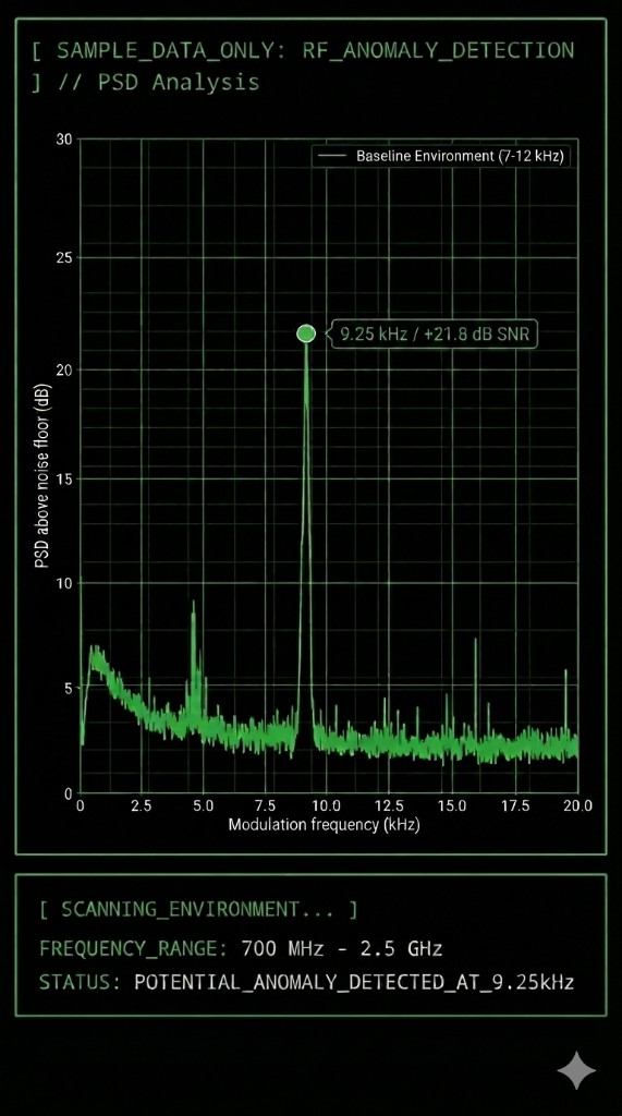
Sample PSD plot, illustrative RF training graphic — PANEL_A // PSD_MAXIMUM (MODULATION SPECTRUM)
FIG_A (sample data): Spectral power on the modulation side of the carrier. For illustration, the biologically relevant region at 9.25 kHz is marked.
Presentation: Modulation frequency (kHz) versus level above the noise floor.
Read as: Look for stable kilohertz peaks that clearly protrude from the noise.

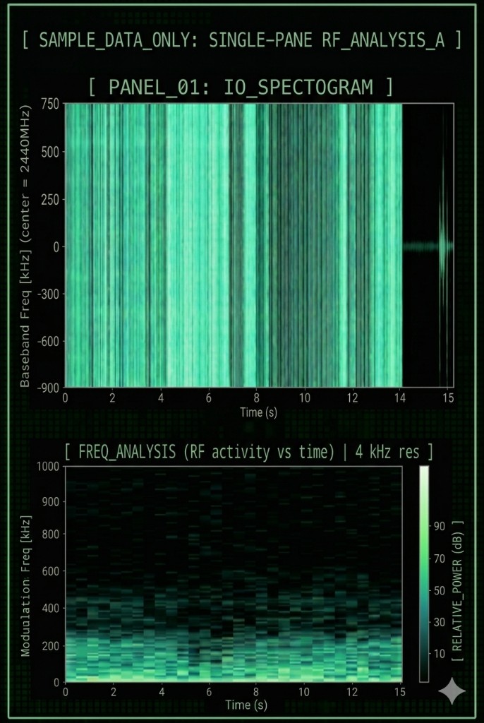
Sample IQ spectrogram and RF activity panels, illustrative — PANEL_B // IQ_SPECTROGRAM (TIME–FREQUENCY MAP)
FIG_B (sample data): Combined IQ spectrogram and general RF activity over time.
Presentation: Time evolution versus frequency distribution.
Read as: Vertical stripes indicate rapid on/off gating of the signal.
Validation: Always compare this view with the envelope FFT. That confirms you are measuring real RF structure, not internal interference from USB packet cadence or computer hardware (host EMI).

Disclaimer: Live signals may vary based on local RF environment and SDR hardware calibration.

[ HARDWARE_INDEX // RETAIL_SEARCH ]

Below is a curated selection of hardware tuned for the analysis workflow described on this page. Depending on your use case—mobile first-pass scanning versus deep signal analysis—the depth of hardware you need varies. Note: when purchasing, always check current seller ratings and technical specifications to ensure full compatibility with the SoapySDR environment.

HackRF One (main SDR)
The Swiss Army knife of RF analysis. It spans a huge frequency range with enough sample-rate headroom to resolve even complex modulation structures cleanly. Ideal if you want one device for broadband scans and detailed IQ captures. Before buying, check board revision and firmware compatibility.
RTL-SDR dongle (budget option)
An affordable entry for first orientation. Ideal for learning the workflow and spotting strong signals in the waterfall. Limited dynamic range makes it better suited to coarse checks; for deep analysis in lower RF bands, combine it with an upconverter.
Wideband antenna (first scan)
The all-round choice for a first overview. Sweep wide frequency spans quickly for anomalies when the target source is still unknown. For precise measurements and maximum signal purity, switch in step two to an antenna tuned to the band of interest.
Directional UHF antenna
Use this when you already have a suspected band and want direction hints. By rotating the antenna and comparing signal strength, you can estimate where the source is likely located. This is practical for narrowing search area before any deeper technical interpretation.
Shielded SMA cables & adapters
The weakest link in the chain. These parts look inconspicuous but decide the purity of your data. High-quality shielding and accurate 50-ohm paths stop interference from laptops, USB ports, or power supplies from coupling straight into the signal path. Keep cable runs as short as possible and avoid unnecessary adapter junctions to minimize signal loss.
USB isolator (noise control)
The barrier against computer-side noise. It breaks electrical ground loops and isolates power between the PC and SDR receiver. Essential for validation: if suspicious trace lines vanish when you change USB ports or use an isolator, you were probably seeing internal hardware artefact—not real RF.
HF upconverter
Frequency extension for the low-frequency range. Many SDRs are unstable or inaccurate at very low HF. An upconverter shifts those signals into a higher, stable operating band of your receiver. Indispensable if you want clean, repeatable analyses below your device's native cutoff frequency.

Affiliate notice: the retailer search links above point to Amazon and include this site’s Associates tag when configured. Qualifying purchases may earn a commission at no extra cost to you.